Model Selection for Bayesian Autoencoders

A Bayesian autoencoder (BAE) places uncertainty over its encoder and decoder weights, making the weight prior a central modeling choice. We choose that prior by matching the distribution of its outputs to reference images, then infer the weights and fit a density model in the learned latent space. Across small image datasets, this improves reconstruction scores and generated samples relative to standard weight priors and several autoencoder baselines.

Making prior knowledge visible

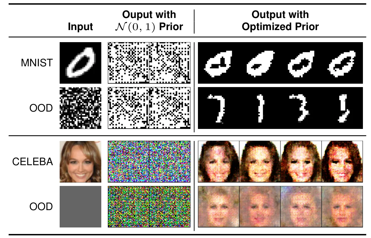
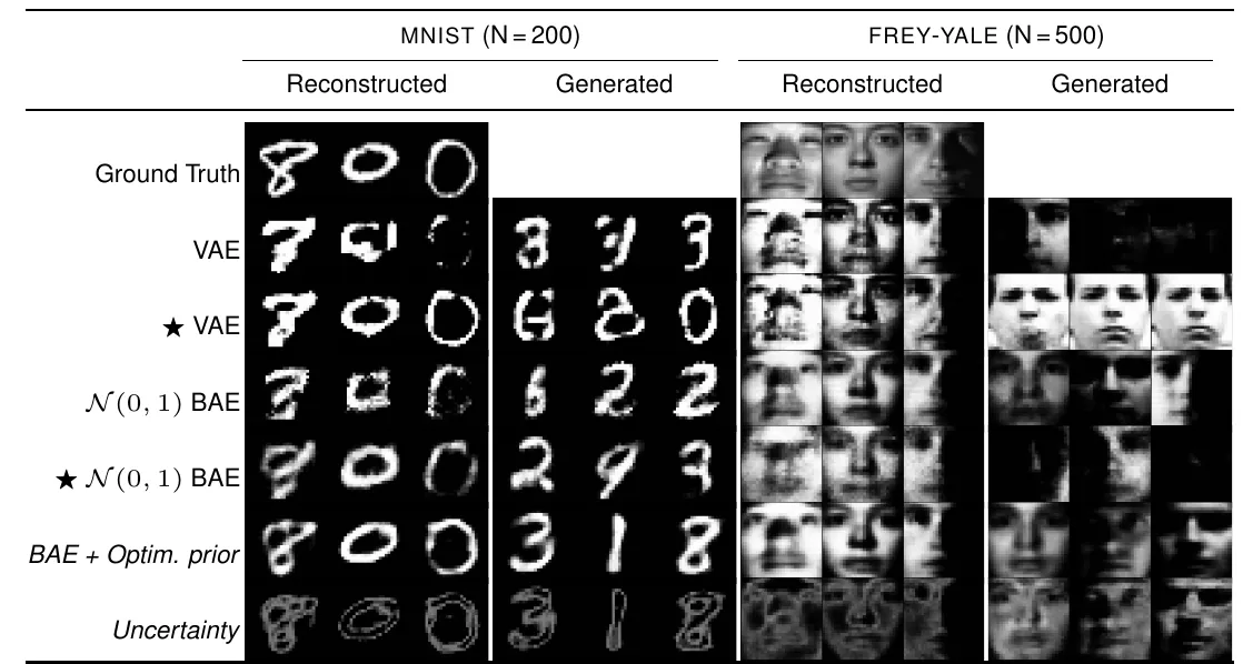
The nonlinear encoder–decoder mapping makes a Gaussian weight prior difficult to interpret. Standard normal weights produce noise-like images; optimized priors produce recognizable structure, including for out-of-distribution inputs.

We use independent Gaussian weights and biases, sharing their means and variances within each layer $l$:

$$p(w_l)=\mathcal N(w_l;\mu_{l_w},\sigma_{l_w}^2), \qquad p(b_l)=\mathcal N(b_l;\mu_{l_b},\sigma_{l_b}^2).$$

These layerwise parameters form $\psi$. Reparameterized samples let gradients reach $\psi$ through both networks and the observation likelihood. For reconstruction, the targets $\mathbf y$ equal the inputs $\mathbf x$. We write distributions over reconstruction targets with conditioning on these inputs left implicit.

Our functional-prior study matches neural-network function samples to a Gaussian-process prior.

Matching distributions through one-dimensional projections

Empirical Bayes motivates selecting $\psi$ through the marginal $p_\psi(\mathbf y)$, which integrates over weights and network outputs. For a fixed data distribution $\pi$, maximizing expected log marginal likelihood is equivalent to minimizing Kullback–Leibler (KL) divergence:

$$\arg\max_\psi\mathbb E_{\pi}[\log p_\psi(\mathbf y)] = \arg\min_\psi\operatorname{KL}[\pi\|p_\psi].$$

Both density evaluation and empirical KL estimation are difficult here. We use distributional sliced-Wasserstein distance as a sample-based surrogate:

$$\begin{aligned} \psi^\star&=\arg\min_\psi DSW_2(p_\psi,\pi),\\ DSW_2(p_\psi,\pi) &=\sup_{\sigma\in\mathbb M_C} \left[\mathbb E_{\boldsymbol\theta\sim\sigma} W_2^2\!\left(\mathcal R p_\psi,\mathcal R\pi\right) \right]^{1/2}. \end{aligned}$$

Here $\mathcal R$ projects each distribution along the unit direction $\boldsymbol\theta$, and $W_2$ measures the Wasserstein distance between the resulting one-dimensional distributions. The admissible direction distributions $\mathbb M_C$ satisfy a constraint, controlled by $C$, that encourages directional diversity. Sorting projected samples gives the one-dimensional transport cost. A learned mapping searches for informative directions while the prior parameters minimize their discrepancy. Model samples include likelihood noise after the autoencoder output. The implementation uses 1,000 projections and 32 prior weight samples per input.

Posterior inference and latent density estimation

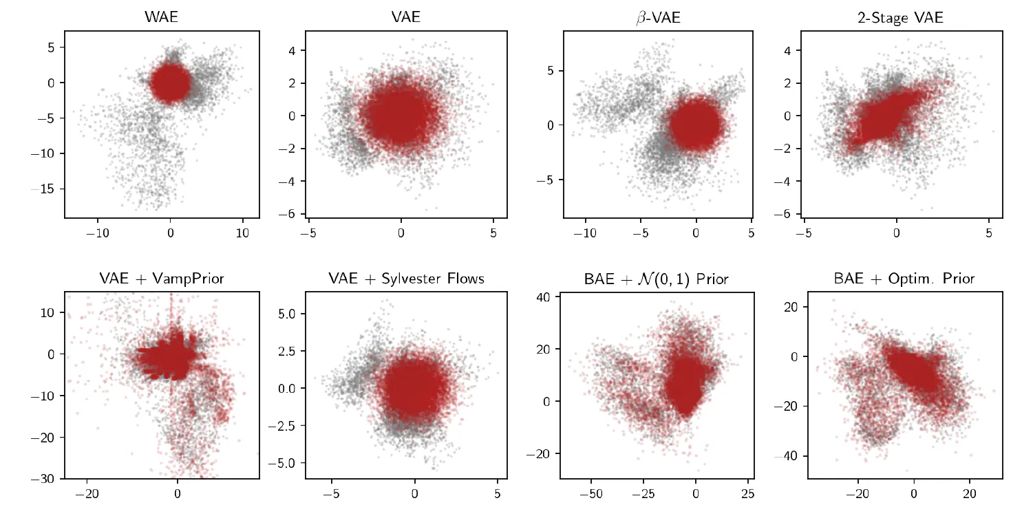
After prior optimization, stochastic gradient Hamiltonian Monte Carlo approximates the weight posterior. We retain 32 samples after burn-in and thinning. To generate images, we fit a Dirichlet process mixture $p_\vartheta(\mathbf z)$ to posterior-mean encoder representations. Its mixture complexity adapts to the data. Generation then uses

$$\mathbf z_{\mathrm{new}}\sim p_\vartheta(\mathbf z), \qquad \mathbf f_{\mathrm{new}} =\mathbb E_{p(\mathbf w_{\mathrm{dec}}\mid\mathbf y)} [f_{\mathrm{dec}}(\mathbf z_{\mathrm{new}};\mathbf w_{\mathrm{dec}})].$$

This supplies an explicit sampling distribution over latent codes and averages decoder uncertainty when producing an image.

Transferring information through the prior

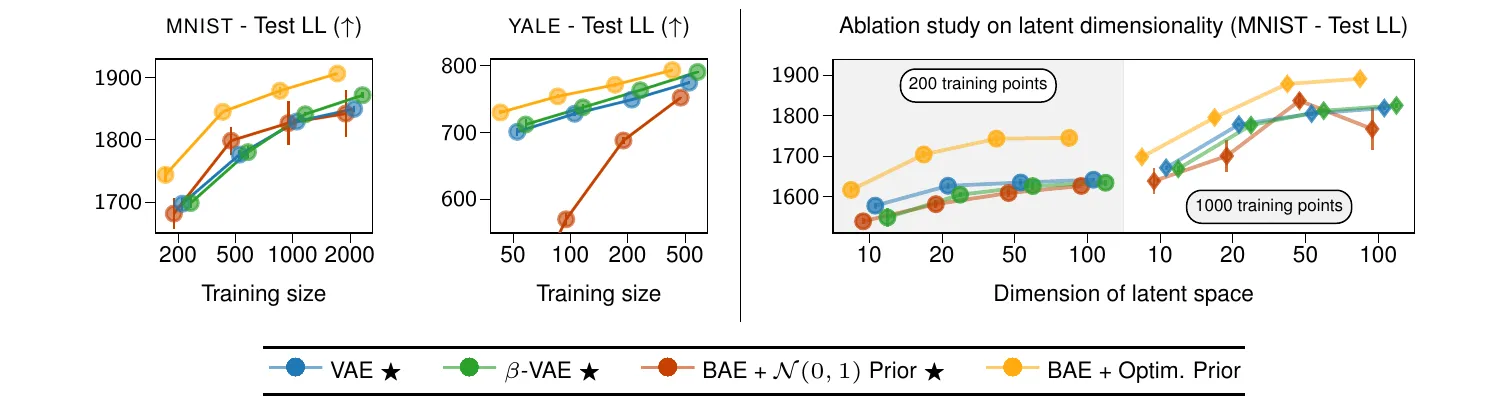
On MNIST, 100 zero digits specify the prior, while posterior inference uses digits one through nine. On Frey–Yale, 1,956 Frey faces specify the prior and Yale faces support inference. These settings test information transfer separately from pooling both datasets for training.

Generating faces with limited observations

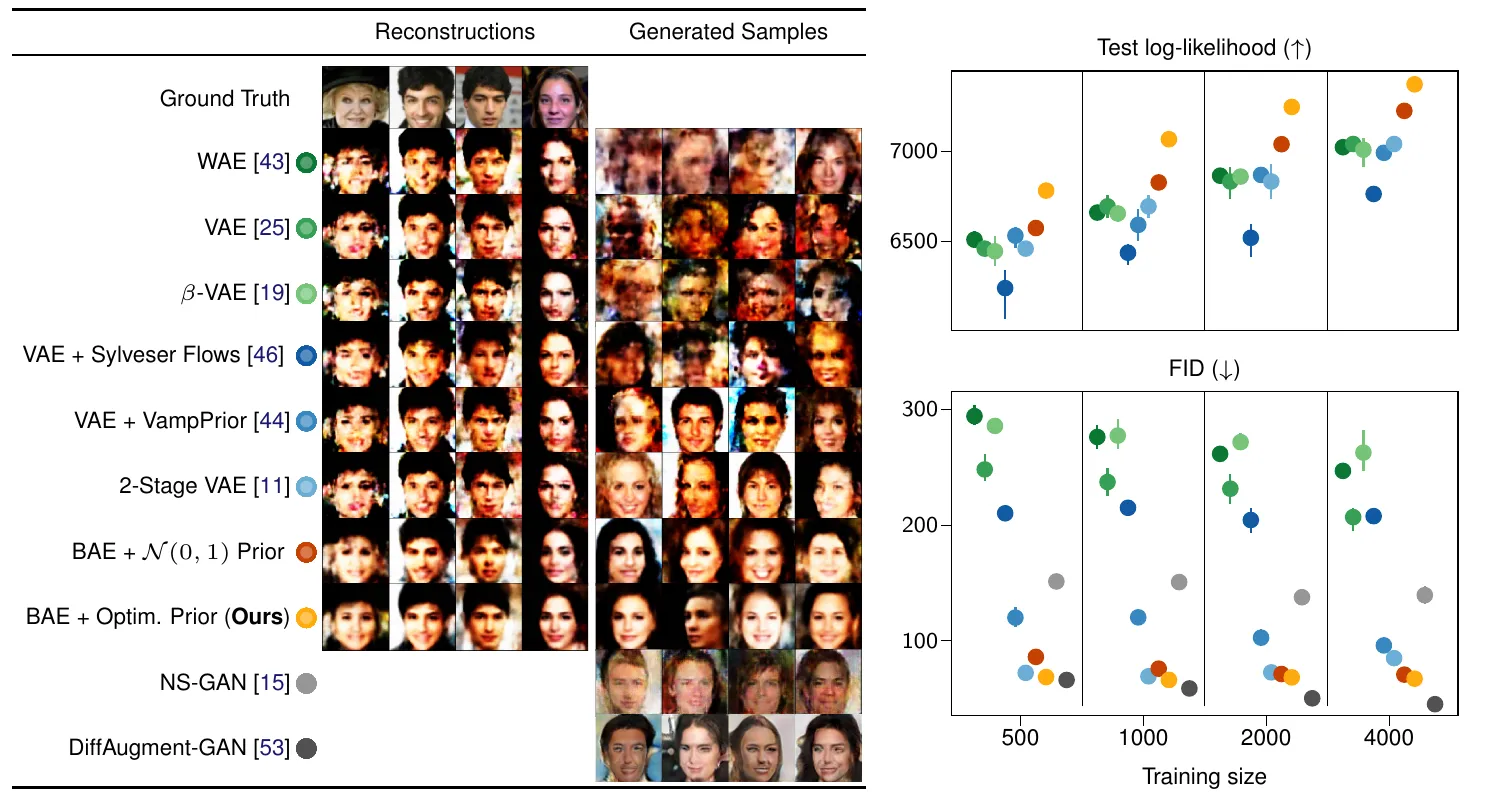
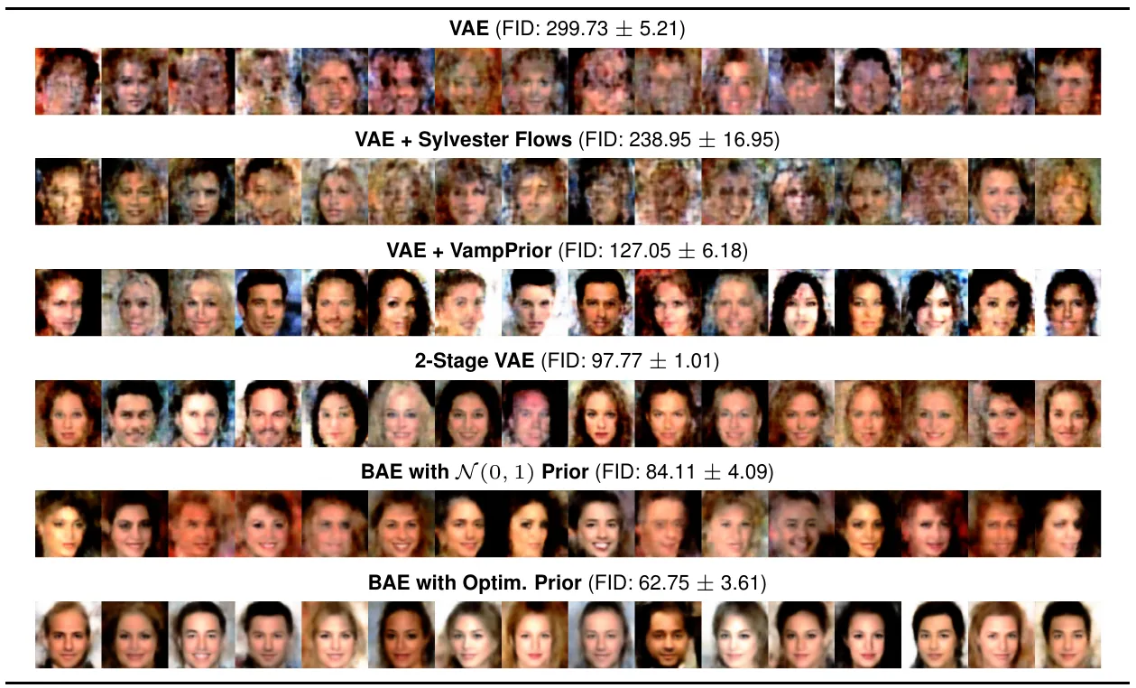
CelebA experiments reserve 1,000 images for prior selection and use 500–4,000 for inference, with four random splits. Images have $64\times64$ resolution and typically 50 latent dimensions. Predictive reconstruction log-likelihood measures reconstruction and uncertainty; Fréchet Inception Distance (FID) evaluates generated-image distributions using 10,000 samples. DiffAugment-GAN achieves lower mean FID at every tested budget; that baseline also uses StyleGAN2 and differentiable augmentation.

Prior selection and posterior tempering

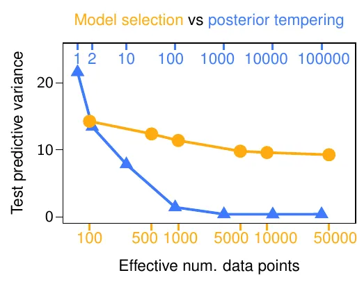
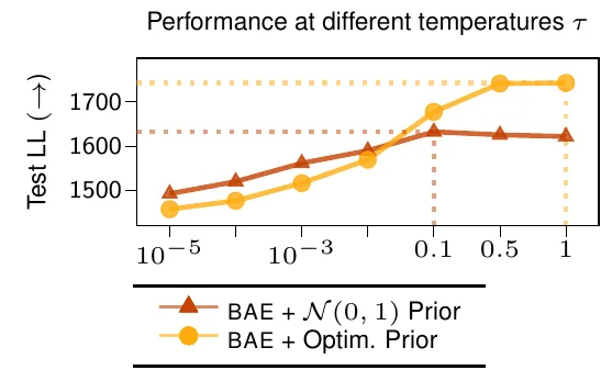
MNIST ablations distinguish changing prior structure from increasing likelihood weight through posterior tempering. At temperature $\tau>0$, tempering raises the likelihood to the power $1/\tau$ while retaining the prior. The optimized prior retains predictive variation as reference data increase, and its best tested reconstruction score occurs at $\tau=1$, the ordinary Bayesian posterior.