How Much is Enough? A Study on Diffusion Times in Score-based Generative Models

A diffusion model learns to reverse the gradual corruption of data into noise. The diffusion horizon determines both how close the corrupted data become to the noise distribution and how much denoising the model must learn. We characterize this trade-off and fit an auxiliary density to the partially corrupted data. This learned starting distribution supports shorter reverse trajectories, with measurable trade-offs between likelihood, image quality, and computation.

Why the diffusion horizon matters

Let $p(\mathbf{x},t)$ be the marginal density of an affine forward diffusion, with $p(\mathbf{x},0)=p_{\mathrm{data}}(\mathbf{x})$. Exact reversal requires its score $\nabla\log p(\mathbf{x},t)$ and samples from $p(\mathbf{x},T)$. In practice, we learn $\mathbf{s}_\theta$ and initialize from a Gaussian $p_{\mathrm{noise}}$. Our evidence lower bound (ELBO) separates these approximations:

$$\begin{aligned} \mathbb{E}_{p_{\mathrm{data}}}\log q(\mathbf{x},T) &\geq \mathcal{L}_{\mathrm{ELBO}}(\mathbf{s}_\theta,T),\\ \mathcal{L}_{\mathrm{ELBO}}(\mathbf{s}_\theta,T) &= C_{\mathrm{data}}-\mathcal{G}(\mathbf{s}_\theta,T)\\ &\quad-\operatorname{KL}\!\left[p(\mathbf{x},T)\,\|\,p_{\mathrm{noise}}\right]. \end{aligned}$$

Here $q(\mathbf{x},T)$ is the generated density and $C_{\mathrm{data}}=\mathbb{E}_{p_{\mathrm{data}}}\log p_{\mathrm{data}}$ is constant. With likelihood weighting $g^2(t)$, where $g$ is the forward diffusion coefficient, the score gap is

$$\mathcal{G}(\mathbf{s}_\theta,T) =\frac12\int_0^T g^2(t)\, \mathbb{E}_{p(\mathbf{x},t)} \left\|\mathbf{s}_\theta(\mathbf{x},t)-\nabla\log p(\mathbf{x},t)\right\|^2\,dt.$$

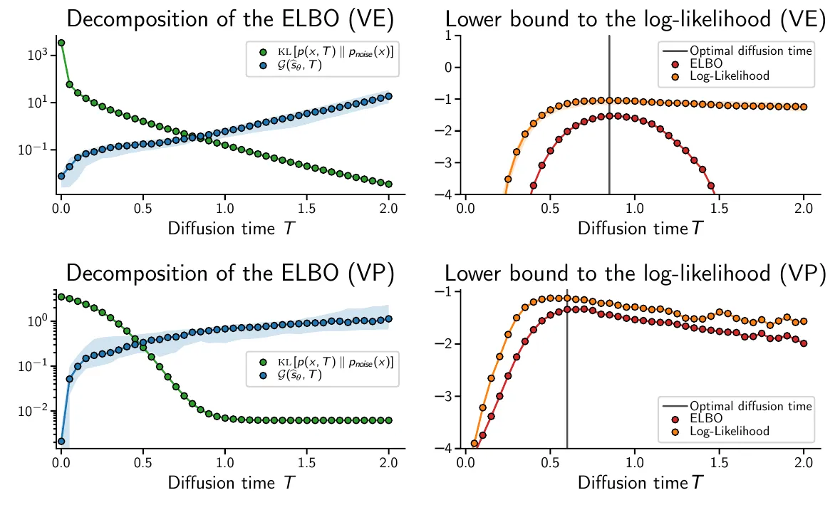
For a fixed score-model family, its globally optimized gap is nondecreasing in $T$. For variance-preserving (VP) and variance-exploding (VE) processes, the Gaussian mismatch decreases with $T$ under the smoothness and finite-KL assumptions of the analysis. These opposing trends make the horizon part of the model choice. For a one-dimensional Gaussian mixture, both processes have finite ELBO-maximizing horizons. The general existence of a finite optimum depends on how the score gap grows.

Learning where reverse diffusion starts

We fit a density $\nu_\phi$ to the endpoint of the shortened forward process. Although $p(\mathbf{x},T)$ is unknown, its samples are available by corrupting training examples with the known Gaussian conditional $p(\mathbf{x},T\mid\mathbf{x}_0)$. The auxiliary model must support sampling and density evaluation:

$$\begin{aligned} \phi^*&=\arg\max_\phi\, \mathbb{E}_{\mathbf{x}_0\sim p_{\mathrm{data}}} \mathbb{E}_{p(\mathbf{x},T\mid\mathbf{x}_0)}\log\nu_\phi(\mathbf{x}),\\ \mathcal{L}^{\phi}_{\mathrm{ELBO}} &=C_{\mathrm{data}}-\mathcal{G}(\mathbf{s}_\theta,T)\\ &\quad-\operatorname{KL}\!\left[p(\mathbf{x},T)\,\|\,\nu_\phi\right]. \end{aligned}$$

Generation samples from $\nu_\phi$, then runs the standard learned reverse diffusion. Its two models can train independently and concurrently. If the auxiliary family contains $p_{\mathrm{noise}}$, globally optimizing $\phi$ weakly improves the endpoint term at the same horizon. With optimal scores, continuity of the auxiliary ELBO, and a baseline optimum $T^*$, the comparison gives

$$\exists\,\tau\leq T^*:\qquad \mathcal{L}_{\mathrm{ELBO}}^{\phi^*}(\widehat{\mathbf{s}}_\theta,\tau) \geq \mathcal{L}_{\mathrm{ELBO}}(\widehat{\mathbf{s}}_\theta,T^*).$$

The bound concerns the ELBO under these optimization assumptions. The useful reduction in horizon depends on how well the auxiliary family fits the endpoint. For the affine diffusion parametrization and scaled auxiliary families used in the analysis, the optimal ELBO depends on the terminal corruption level. This fixes the corruption level as the relevant quantity when comparing a shorter horizon with a faster noise schedule.

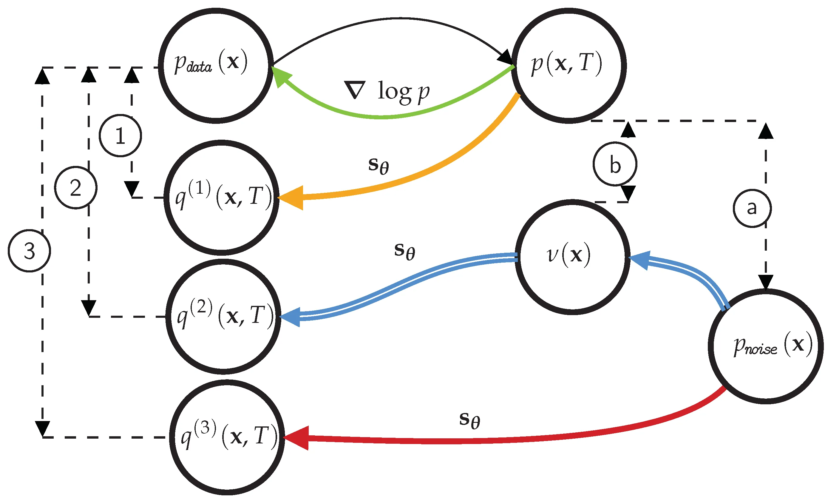
Shorter horizons leave more structure in the endpoint distribution and require greater auxiliary capacity. We use a Dirichlet-process Gaussian mixture on MNIST and the Glow normalizing flow on CIFAR10 and CelebA.

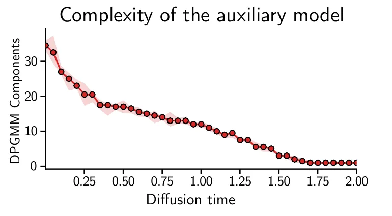
Image quality, likelihood, and sampling cost

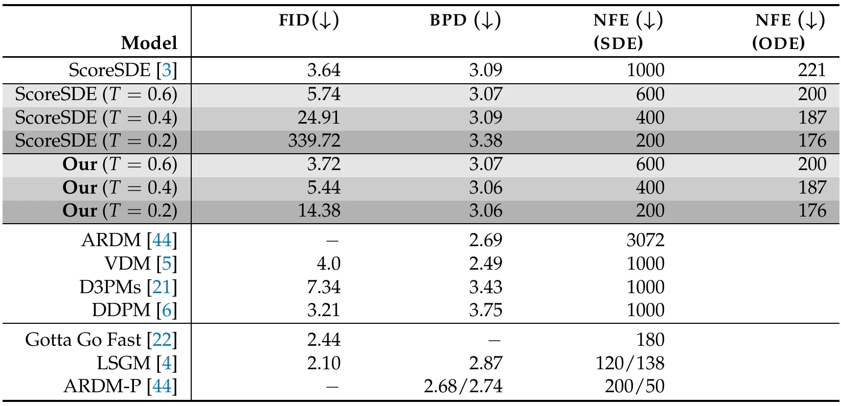
On MNIST and CIFAR10, we keep the VP noise schedule fixed and train the score over $[0,T]$, using a reduced U-Net and NCSN++, respectively. On MNIST, the auxiliary model at $T=0.4$ obtains 1.17 bits per dimension (BPD) with 235 ordinary differential equation (ODE) evaluations; the $T=1$ baseline obtains 1.16 with 300.

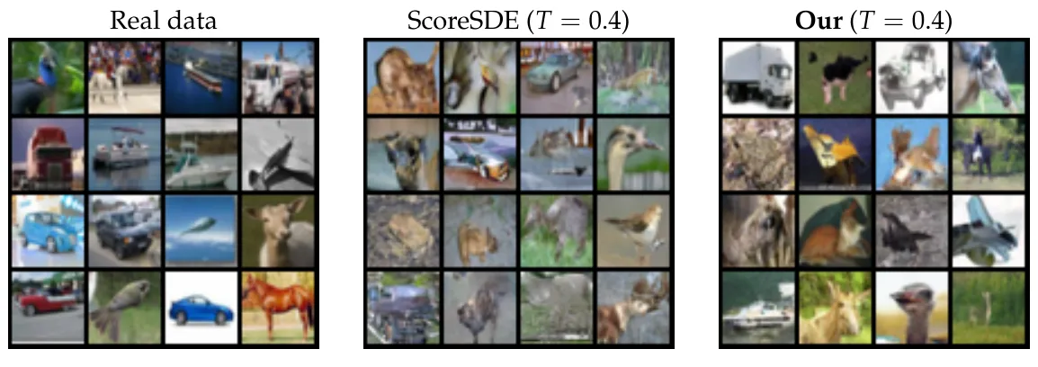
For CIFAR10, $T=0.6$ reduces stochastic sampling from 1000 to 600 neural function evaluations (NFE), with Fréchet Inception Distance (FID) changing from 3.64 to 3.72. At $T=0.4$, the auxiliary model achieves FID 5.44 versus 24.91 for direct Gaussian initialization at the same horizon.

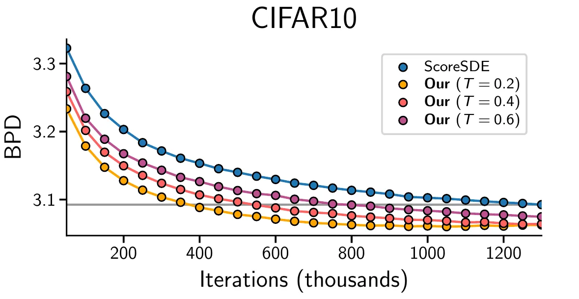
The CIFAR10 training curves reach the baseline's final BPD sooner. In our four-GPU training comparison, the runs take approximately 6.4 days for the baseline, two days for the shortened score model, and 2.3 days for Glow. With resources for concurrent training, the latter two take 2.3 elapsed days.

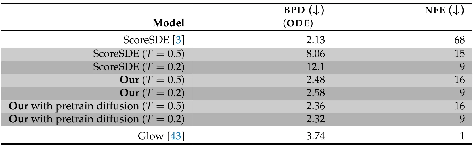
For CelebA at $64\times64$, we use VE diffusion and Glow. Reusing a score pretrained at $T=1$, then sampling at $T=0.2$, gives BPD 2.32 with nine ODE evaluations, versus 2.13 with 68 for the full-horizon baseline.

The likelihood calculation also depends on the sampling dynamics. An approximate probability-flow ODE has its own endpoint distribution; fitting an auxiliary density to those endpoints requires sequential training and yields modest likelihood gains on MNIST. Across these experiments, a shorter diffusion trajectory shifts computation into the auxiliary model. The resulting benefit depends on its capacity to represent the partially corrupted data and on whether training targets stochastic or deterministic endpoints.

For trajectory prediction, our joint trajectory diffusion model uses an informative Gaussian to start reverse sampling at an earlier diffusion time.