Optimizing Diffusion Models for Joint Trajectory Prediction and Controllable Generation
- Diffusion Models
- Computer Vision
Optimal Gaussian Diffusion shortens trajectory sampling, while Estimated Clean Manifold guidance applies control gradients directly to estimated clean trajectories.
Paper ECCV 2024
- UC Berkeley
- EURECOM
- Stellantis
Joint trajectory prediction must represent several road users and the different ways they could interact. Diffusion models can generate these joint futures and steer them toward requested routes or speeds, but repeated denoising and guidance make sampling expensive. We introduce Optimal Gaussian Diffusion (OGD), which starts sampling from an informative Gaussian at an earlier diffusion time, and Estimated Clean Manifold (ECM) guidance, which applies control gradients directly to estimated clean trajectories. On Argoverse 2, the combination improves goal satisfaction while reducing sampling steps and guidance overhead.
Starting closer to the trajectory distribution
Predicting each vehicle independently can combine individually plausible motions into an inconsistent scene. We therefore model the joint future , conditioned on observed motion and map context. Throughout the equations, we omit this conditioning for clarity.
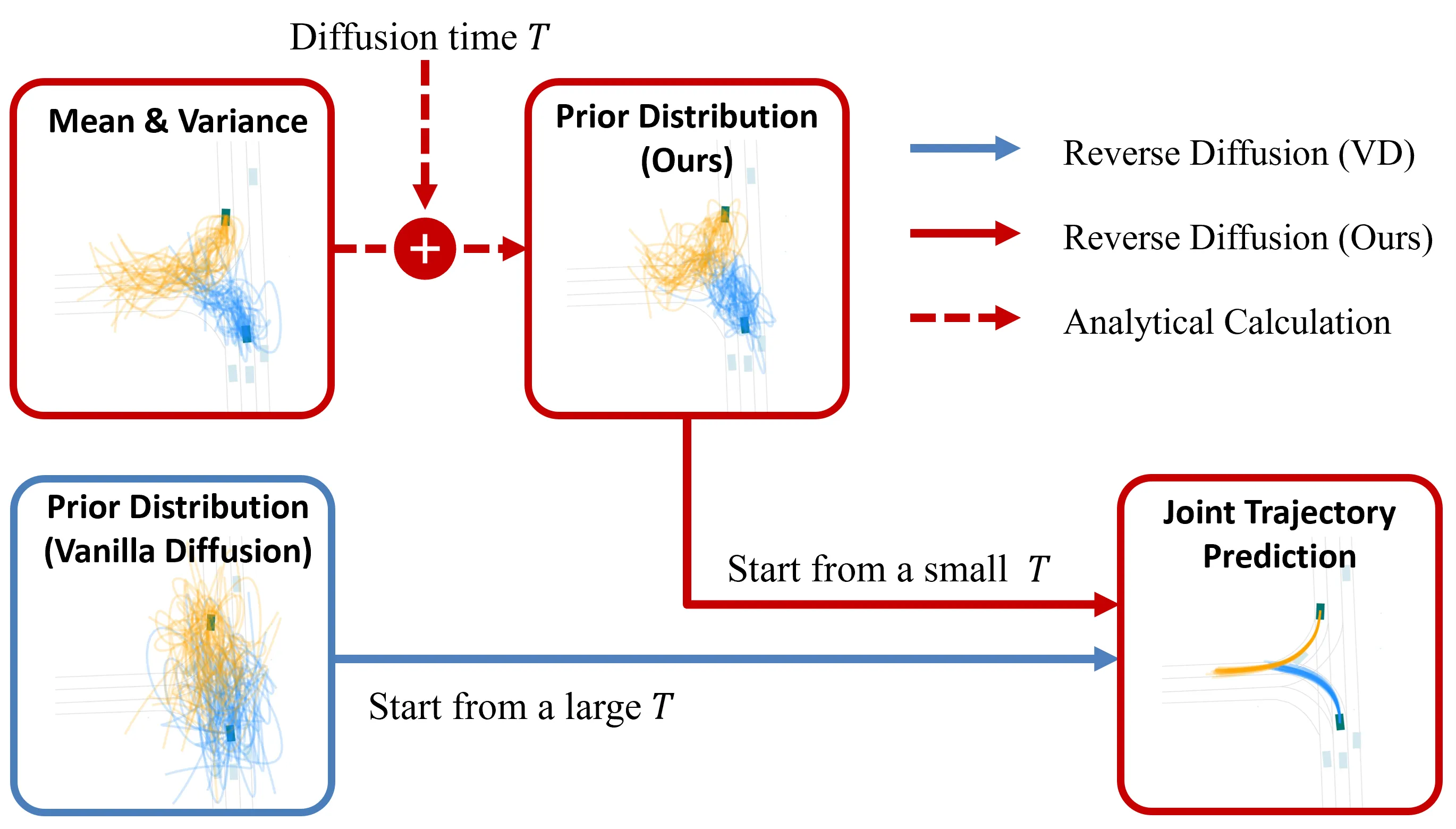
Vanilla diffusion begins reverse sampling from a non-informative Gaussian after enough forward diffusion to erase the data structure. OGD chooses an informative Gaussian for a smaller starting time :
Here is the noisy trajectory distribution, is the perturbation-kernel covariance, and denotes the determinant. For a variance-preserving Gaussian perturbation kernel, the minimizing prior and kernel parameters can be expressed in terms of the data mean and covariance. For joint prediction, the practical construction restricts covariance to blocks for individual agents and estimates these statistics with a pretrained marginal predictor. The denoiser learns the remaining joint dependence, and can be tuned during inference.
Our study of diffusion times examines the broader trade-off between score approximation and reverse-process initialization.
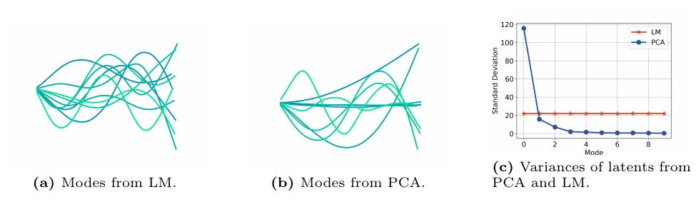
Our implementation uses a frozen QCNet context encoder, attention over agents, maps and marginal predictions, and a learned linear mapping from 120 trajectory coordinates to ten latent dimensions. This representation also regularizes the scale of latent components.
Applying control gradients to clean estimates
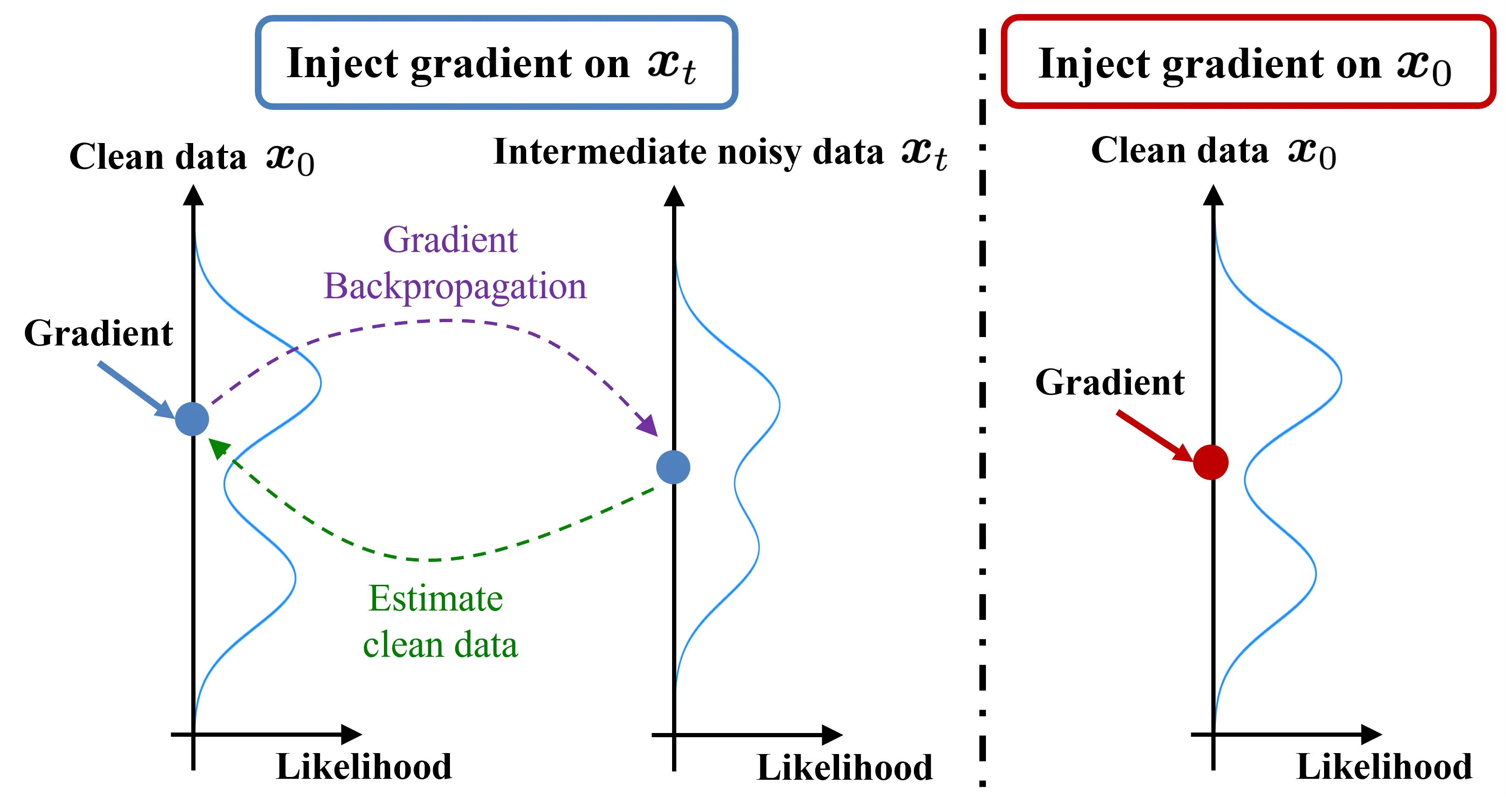
Control costs naturally describe clean trajectories, such as the distance to a requested position. Conventional score-function guidance differentiates that cost through the denoising network. ECM instead treats realism and control as a hierarchical optimization:
The learned density supplies the primary realism objective; encodes the requested behavior. Each iteration first injects noise and estimates a clean trajectory, then reduces the control cost:
The noise predictor is , specifies the noise level, and is the control step size. The update assumes a sufficiently small displacement to limit deterioration of the realism objective. Its control gradient requires differentiation only through the cost. We decrease over iterations and use deterministic noise reuse in the evaluated implementation.
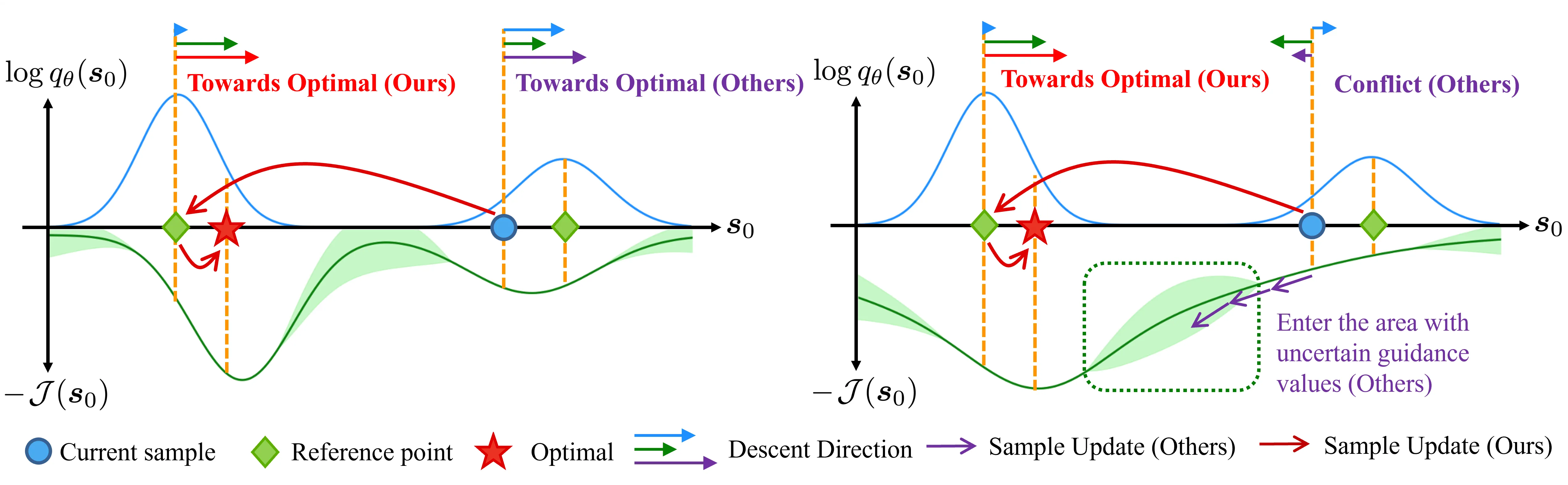
Road topology creates separated trajectory modes. ECM with Reference Joint Trajectories (ECMR) evaluates combinations of marginal predictions and the current clean estimate, chooses a low-cost reference, and then applies guidance. This gives the optimizer a starting point near another candidate mode.
Prediction, control, and measured cost
We evaluate on Argoverse 2 with five seconds of observations and six seconds of prediction. Against an architecture-matched vanilla diffusion model starting at , OGD at matches or improves all four evaluated prediction metrics. With DDIM stride ten, these horizons correspond to four and fifty sampling steps.
Controllable generation uses 128 samples and goals on ground-truth routes (GT) or combinations of marginal routes (U), with normal speed, deceleration, and acceleration settings. Joint Final Displacement Error (JFDE) measures goal satisfaction; Joint Route Deviation Error (JRDE) measures route adherence. We compare against Next Noisy Mean (NNM) guidance and Score Function (SF) guidance, with tuned control step sizes.
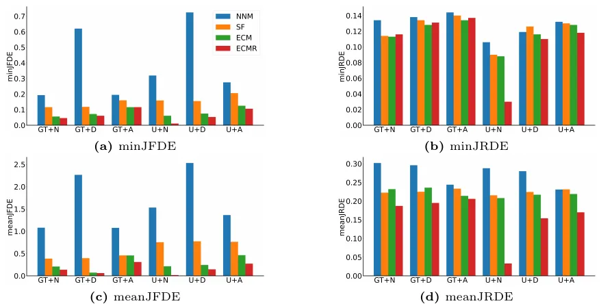
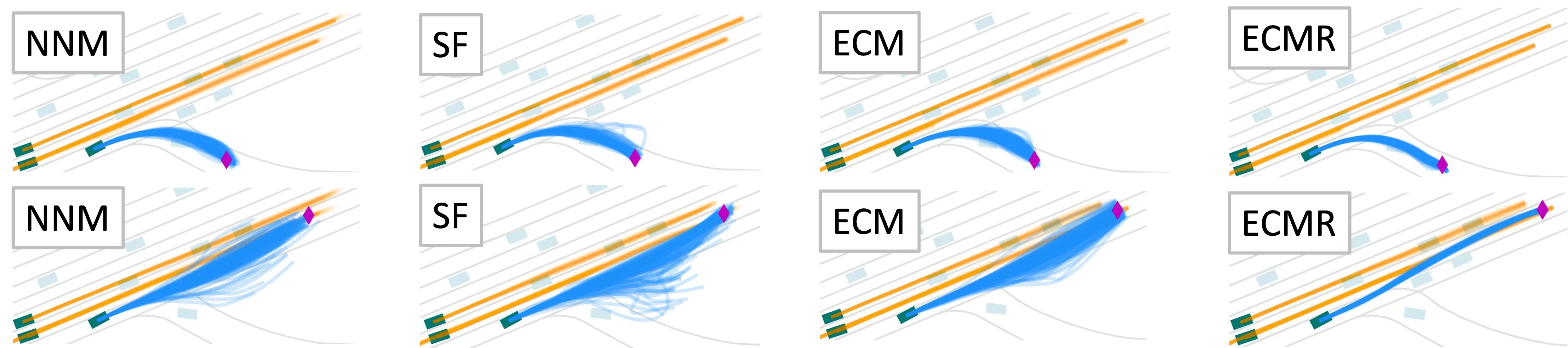
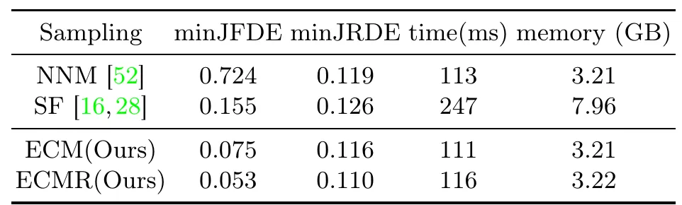
For U with deceleration, OGD+ECMR uses ten DDIM steps and attains minJFDE 0.053, versus 0.538 for vanilla diffusion with score-function guidance and fifty steps. The corresponding minJRDE values are 0.110 and 0.158.
Selecting the control step size
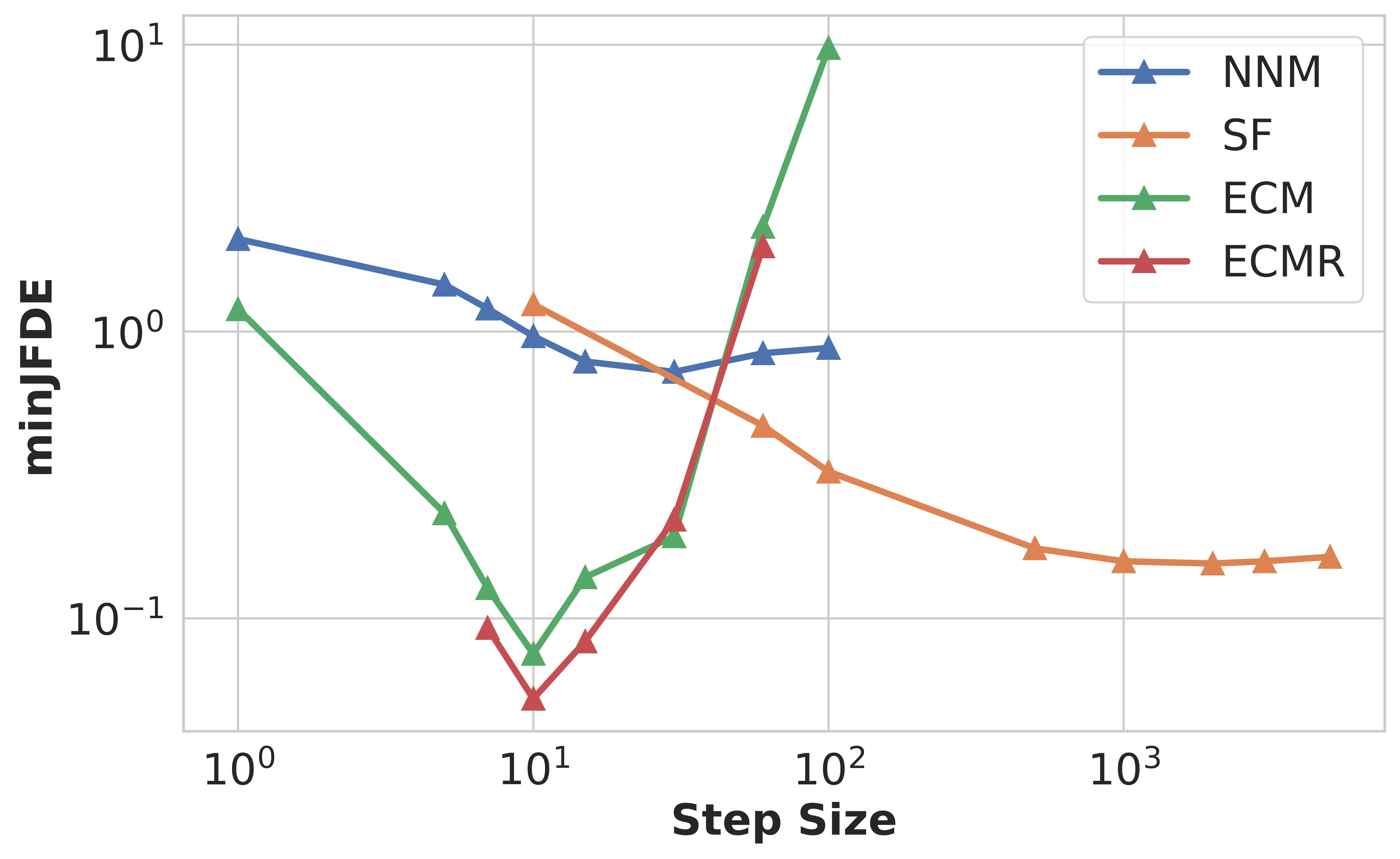
We tune the guidance step size by grid search to minimize goal error.
These experiments measure realism through route adherence in recorded scenes. The marginal predictor supplies both the statistics used to initialize OGD and the candidate routes used by ECMR, so its predictions influence generation quality and the available control choices.