DrivingVoxels: Compositional Sparse Voxel Rasterization for Dynamic Driving Scene Reconstruction
- Computer Vision
DrivingVoxels reconstructs dynamic driving scenes with separate sparse voxel octrees for the background and moving objects, composed in a single rendering pass.
Paper BMVC 2026
- Huawei Paris Research Center & EURECOM
- Huawei Paris Research Center
- EURECOM
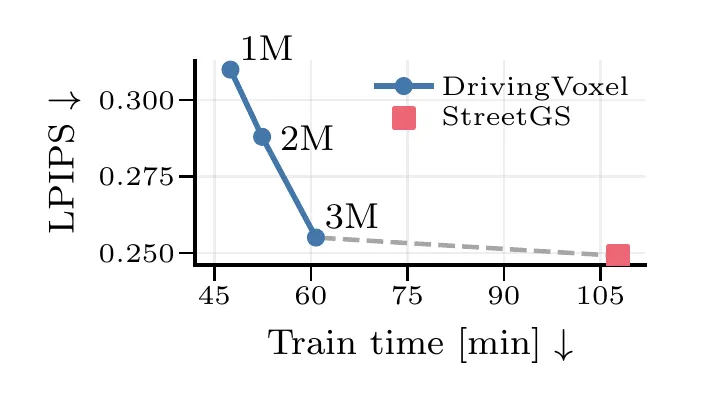
Reconstructing a driving scene requires consistent geometry for both the stationary environment and independently moving actors. We introduce DrivingVoxels, an explicit sparse voxel representation with a separate octree for each rigid object and one for the background. A single rendering pass composes their contributions in depth order. On ten PandaSet sequences, this construction improves geometric reconstruction over the reproduced Gaussian-splatting baselines while reducing training time, with a trade-off in perceptual detail.
The work is accepted at BMVC 2026.
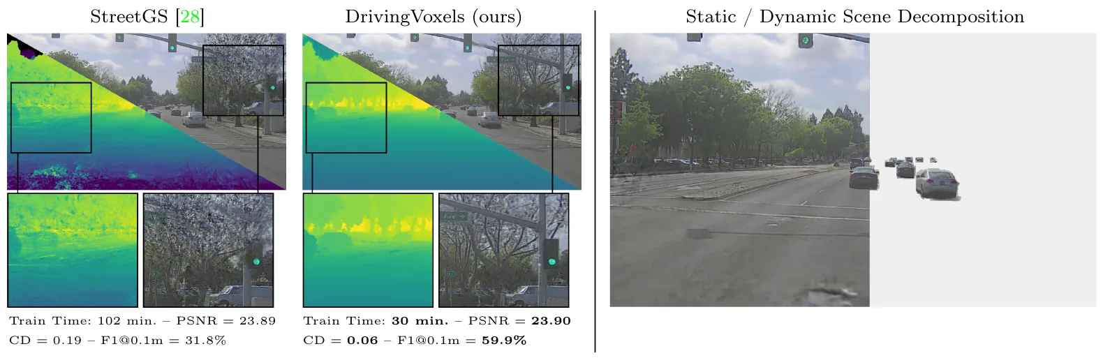
Motion in separate coordinate frames
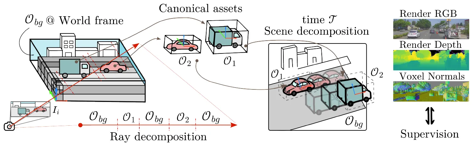
A static voxel grid fixes its spatial partition, making independently moving objects difficult to represent. We retain sparse voxel rasterization inside each octree and solve composition between octrees along camera rays.
The background octree lives in world coordinates. Object has a canonical octree and a tracked rigid transformation at time . Each leaf voxel stores spherical-harmonic appearance coefficients and eight corner densities, interpolated within the voxel. A spherical environment map represents the sky.
LiDAR-based geometry initialization
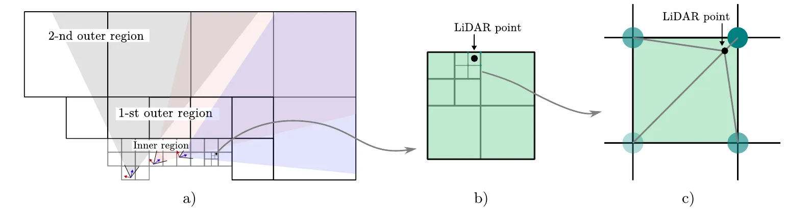
We prune background voxels outside the training-camera frustums or below the height threshold, then subdivide near LiDAR points. This allocates resolution around observed surfaces while retaining coarse empty space. Initial raw corner density depends on the nearest LiDAR distance :
Here is the minimum voxel size, , and . The smooth prior seeds density near measurements while leaving densities trainable. Object octrees instead start from uniform grids bounded by annotated boxes, avoiding LiDAR initialization errors from temporal misalignment.
Ray accumulation across multiple octrees
For a ray with origin , direction , and distance , we sort object-box entry and exit distances. Background intervals use world coordinates; object intervals use . The renderer carries accumulated color, depth, normals, and residual transmittance between intervals. After voxel integration, sky compositing gives
is the fraction of light transmitted through all visited volumes. It weights the sky contribution, preserving occlusion across coordinate boundaries.
The joint training objective combines image and geometric evidence:
The coefficients weight color reconstruction, sparse LiDAR depth, dense pseudo-normal alignment, and a sky-transmittance penalty. Background subdivision stops when SSIM improvement plateaus, followed by pruning and refinement.
Image quality and geometric reconstruction
The evaluation uses the front camera of ten PandaSet sequences, with 40 training and 40 held-out frames per sequence. Camera poses and object tracks are fixed, and actors are modeled as rigid. Calibration and tracking errors affect reconstruction accuracy. Geometry is compared against accumulated LiDAR. The adaptive configuration achieves 0.242 m Chamfer distance and 65.6% F1 at 0.1 m, versus StreetGS's 0.605 m and 54.8%. Mean training time is 0.41 hours versus 1.80 hours on RTX 3090-equivalent hardware; StreetGS renders faster, at 57 versus 26 FPS.
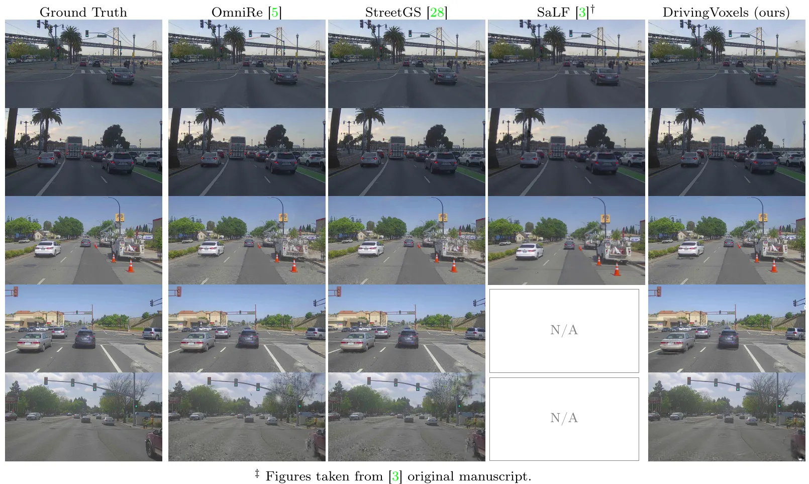
On five-sequence ablations at 20,000 iterations, removing LiDAR subdivision worsens perceptual and geometric metrics. Binary density initialization performs similarly to the smooth prior. Removing depth supervision increases Chamfer distance from 0.231 to 0.644 m; removing normal supervision reduces F1 from 66.3% to 49.0%.

Editing reconstructed actors
Separate octrees support actor removal, pose changes, and replacement after reconstruction.
