Understanding in-context learning in transformers

A transformer can infer a new task from examples in its prompt while its parameters remain fixed. For noiseless linear regression, a linear self-attention layer can implement a least-squares gradient step by updating its token coordinates. We reproduce the construction of von Oswald et al. and find close agreement between pretrained linear attention and the gradient-step predictor. Agreement holds for both predictions and input gradients when the comparison uses the appropriate learning rate.

Our study of query initialization examines this correspondence when regression tasks share a non-zero prior mean.

Learning a procedure across regression tasks

Each task draws a $D$-dimensional weight vector $\boldsymbol w\sim\mathcal N(\boldsymbol 0,\alpha^2\boldsymbol I_D)$ and independent inputs from $\mathcal U(-1,1)^D$. Its labels are $y_i=\boldsymbol w^\top\boldsymbol x_i$. A prompt contains $C$ labeled examples and an unlabeled query. We train shared transformer parameters $\boldsymbol\theta$ by minimizing the expected query error:

$$\begin{aligned} P_C&=[\{\boldsymbol x_i,y_i\}_{i=0}^{C-1},\boldsymbol x_{\mathrm{query}}],\\ \mathcal L(\boldsymbol\theta) &=\mathbb E\!\left[ \left(f(\boldsymbol\theta,P_C)-y_{\mathrm{query}}\right)^2 \right]. \end{aligned}$$

The expectation covers both functions and inputs. Fresh tasks are generated during pretraining; evaluation uses 10,000 fixed tasks from the same distributions. A successful model therefore acquires a procedure that uses a new prompt to predict its query output.

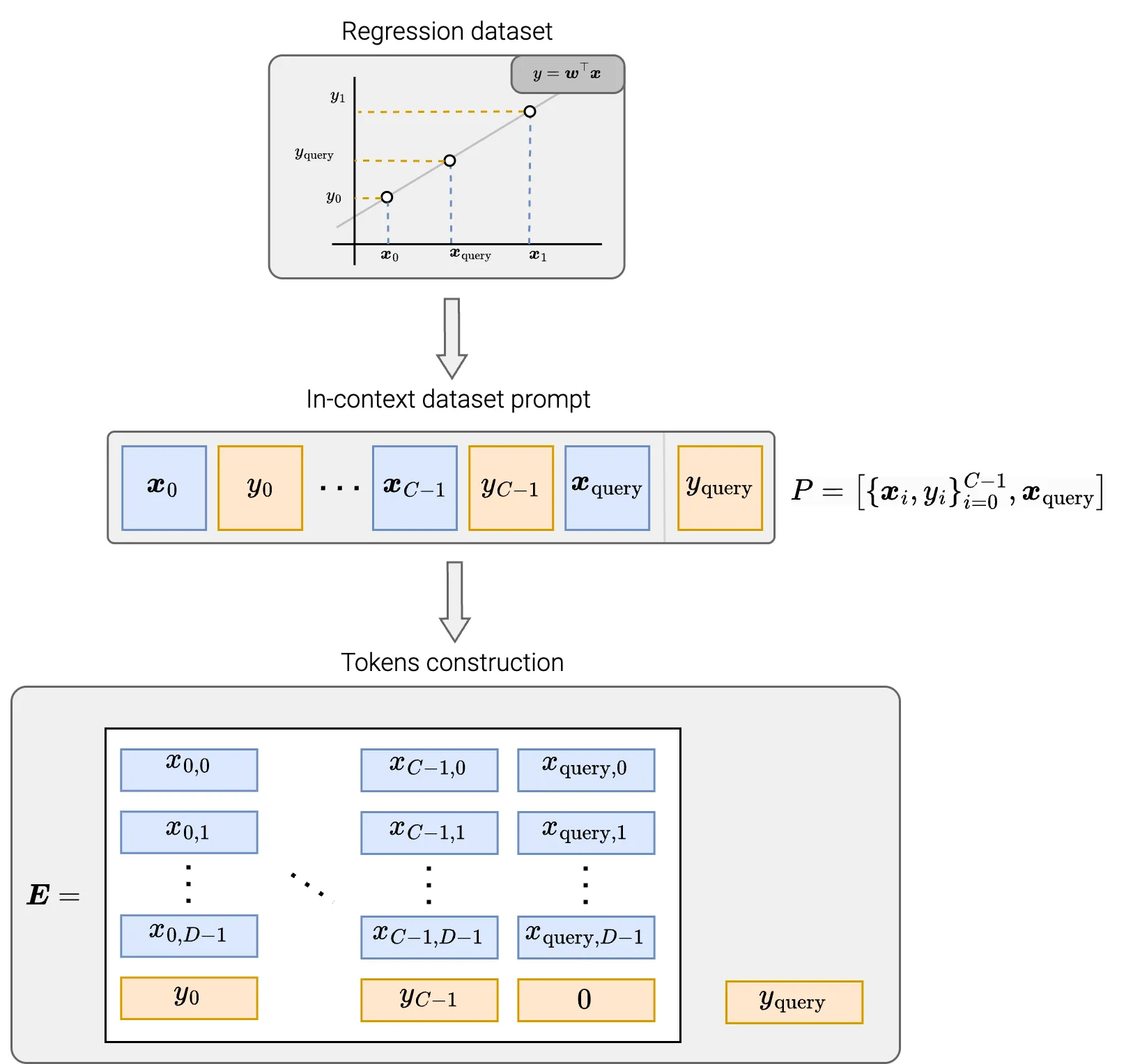
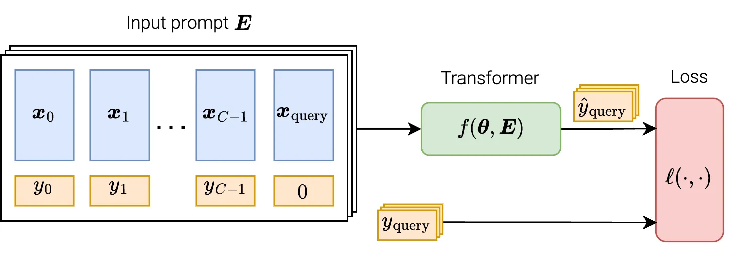
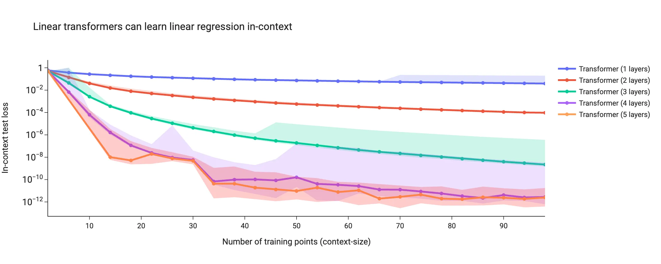
We compare models with one to five layers and contexts from 2 to 100 examples. Both softmax and linear attention improve with context and depth in these experiments. The linear model removes softmax, normalization, feed-forward blocks, and additional embeddings, retaining single-head attention and residual updates.

Encoding a gradient step in the tokens

For a single regression task, least squares and one gradient step from $\boldsymbol w_0=\boldsymbol 0$ give

$$\begin{aligned} \mathcal L_{\mathrm{lin}}(\boldsymbol w) &=\frac{1}{2C}\sum_{i=0}^{C-1} (\boldsymbol w^\top\boldsymbol x_i-y_i)^2,\\ \boldsymbol w_1 &=\boldsymbol w_0-\eta\nabla\mathcal L_{\mathrm{lin}}(\boldsymbol w_0) =\frac{\eta}{C}\sum_{i=0}^{C-1}y_i\boldsymbol x_i. \end{aligned}$$

Here $\eta$ is the regression learning rate. The key observation is that the same prediction can be encoded by changing token coordinates while keeping the attention parameters fixed. Choose keys and queries that retain the input coordinates, values that extract the negative labels, and a projection that supplies the factor $\eta/C$, including the attention normalization. The resulting token update is

$$\begin{aligned} \boldsymbol e'_j &=\begin{pmatrix}\boldsymbol x_j\\y_j\end{pmatrix} +\begin{pmatrix} \boldsymbol 0\\ -\dfrac{\eta}{C}\displaystyle\sum_{i=0}^{C-1} y_i\boldsymbol x_i^\top\boldsymbol x_j \end{pmatrix},\\ \widehat y_{\mathrm{query}} &=-\bigl(\boldsymbol e'_{\mathrm{query}}\bigr)_{D+1} =\boldsymbol w_1^\top\boldsymbol x_{\mathrm{query}}. \end{aligned}$$

The query token starts at $(\boldsymbol x_{\mathrm{query}},0)$; its actual label stays outside the attention computation. Keys and values use context tokens only. This construction uses noncausal attention and a negative readout of the query's last coordinate. Several parameter factorizations implement the same operation.

Comparing learned predictions and gradients

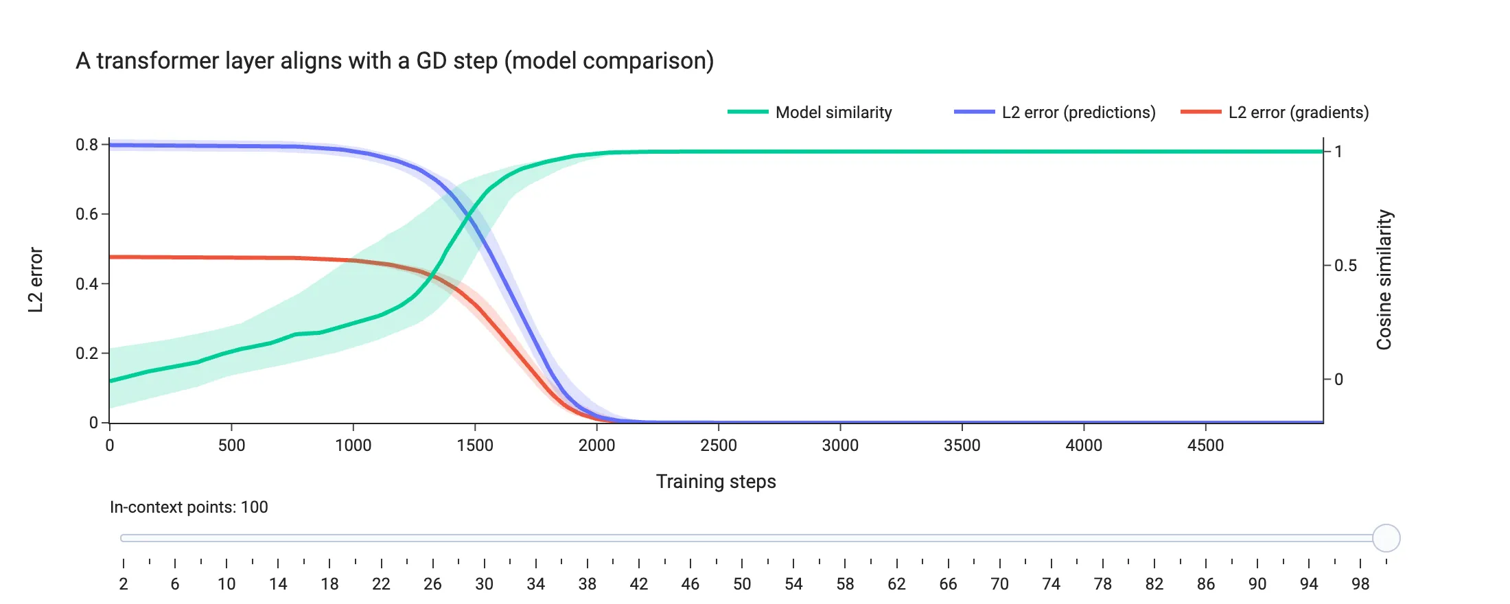
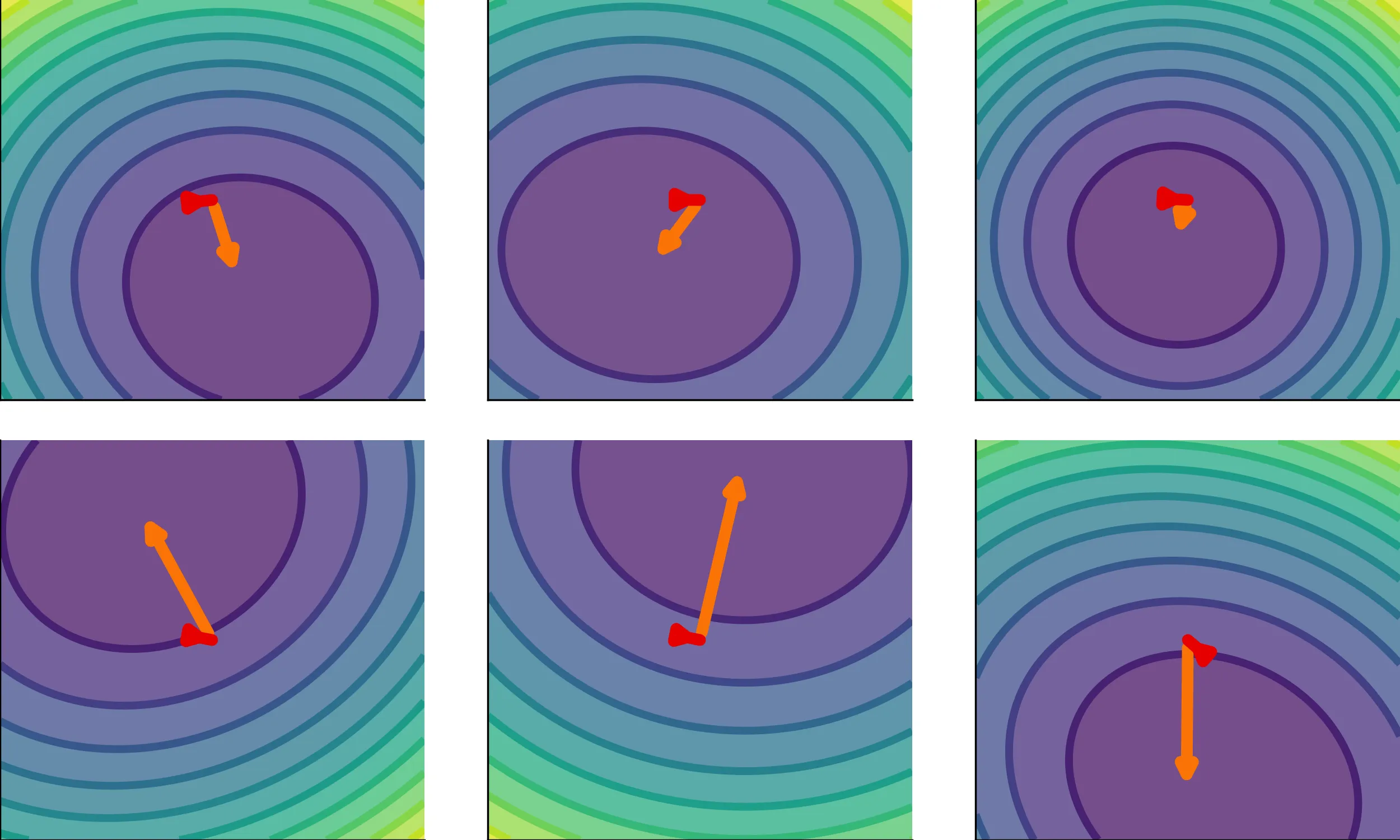
We train a single layer and compare it with the explicit gradient-descent construction. Across the tested context sizes, their losses approach each other. We also measure squared prediction differences, differences between gradients with respect to the query input, and their cosine similarity. These additional comparisons directly examine the functions computed on sampled tasks.

Identifying the effective learning rate

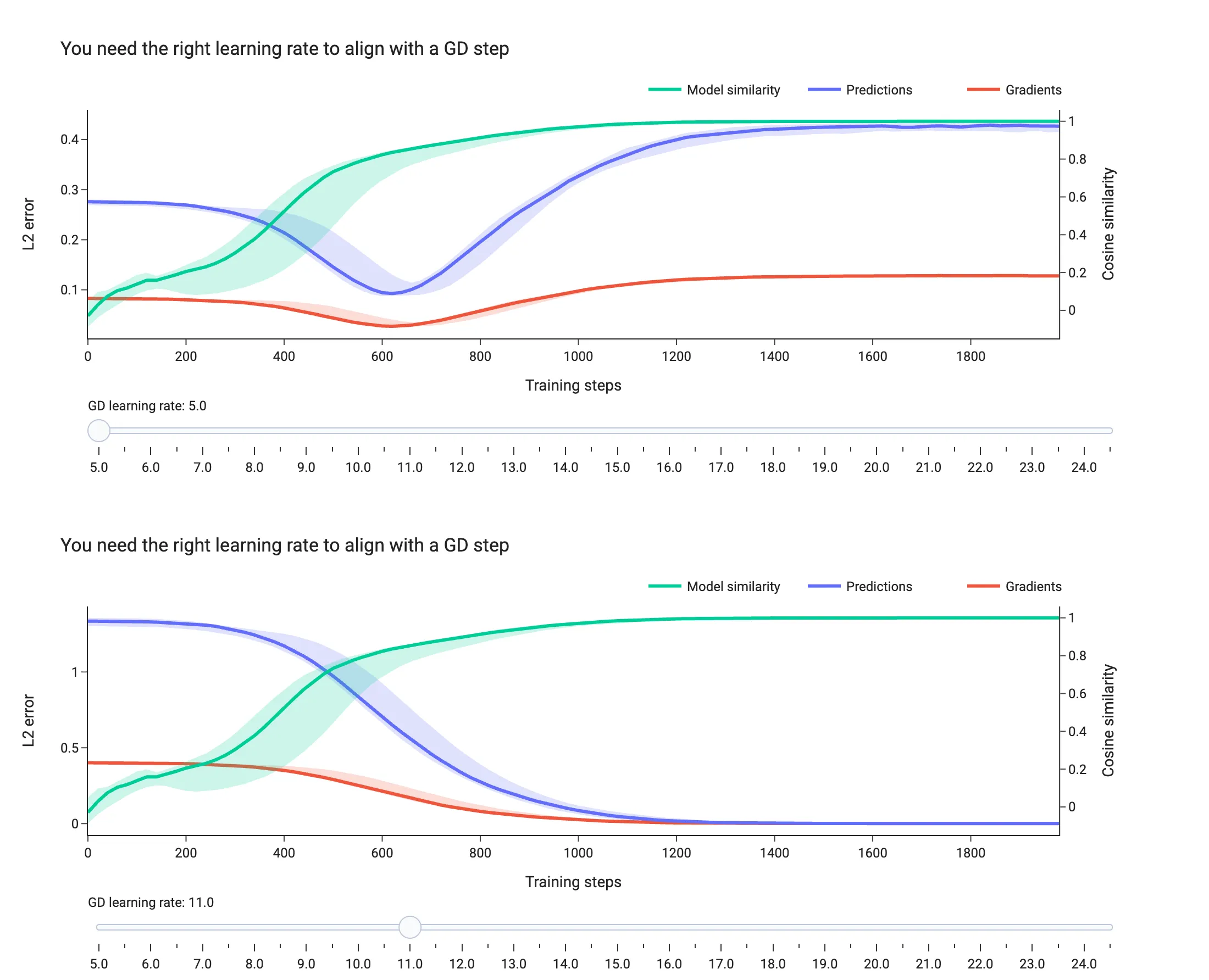
Agreement between predictions and gradients requires the correct scale as well as direction. For zero initialization, define $s_n$ from task $n$'s context. Minimizing the quadratic empirical query loss over $N$ labeled tasks gives

$$\begin{aligned} s_n&=\sum_{i=0}^{C-1}y_i^{(n)} (\boldsymbol x_i^{(n)})^\top\boldsymbol x_{\mathrm{query}}^{(n)},\\ \eta^*&=C\frac{\sum_{n=0}^{N-1}y_{\mathrm{query}}^{(n)}s_n} {\sum_{n=0}^{N-1}s_n^2}. \end{aligned}$$

The denominator must be nonzero. This formula selects a comparison learning rate from labeled tasks; inference then uses the fixed rate. It agrees with line search in our experiments and explains how pretraining can absorb an effective step size into the attention matrices.

Stabilizing repeated gradient steps

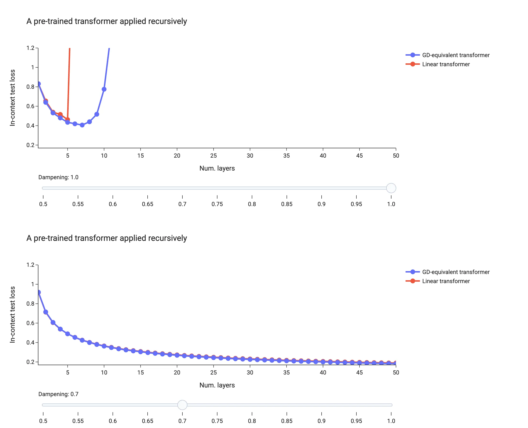
Recursively applying a layer trained for one step can diverge. Multiplying each residual update by a damping factor $\lambda$ rescales its effective learning rate. In the illustrated experiment, $\lambda=0.70$ stabilizes recurrence, while $\lambda=1$ diverges.

Unidirectional LSTMs align less closely with the gradient-descent baseline in the same regression tasks. Deeper bidirectional LSTMs produce predictions closer to this baseline, with residual differences in the computed functions. For the simplified noncausal attention model, the agreement in predictions and input gradients, together with its dependence on learning rate, supports the gradient-step account of adaptation to noiseless linear functions.