From predictions to confidence intervals: an empirical study of conformal prediction methods for in-context learning
- Large Language Models
- Uncertainty Quantification
We combine conformal prediction with in-context learning to construct prediction intervals for noisy linear regression, using transformer predictions in place of repeated model fits.
Paper AABI 2025
- PSL Research University
- EURECOM
- Stellantis
A transformer can learn a regression task from examples in its prompt, while its parameters remain fixed. We use this in-context learning (ICL) ability to construct prediction intervals with conformal prediction. Transformer evaluations replace the repeated regression fits inside full conformal prediction. On synthetic noisy linear regression, the resulting intervals approach the requested 90% coverage and behave similarly to a ridge-based conformal reference, with comparable inference times in our implementation.
Why prediction intervals require candidate responses
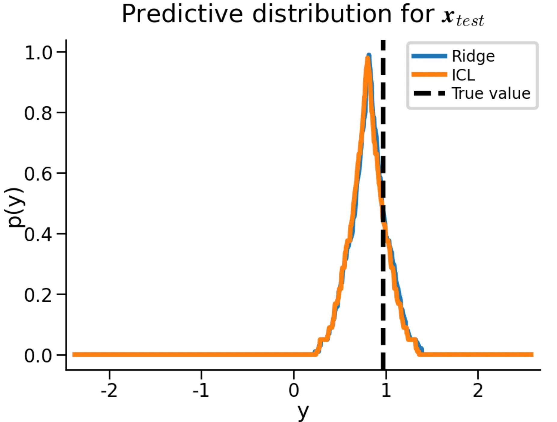
A point prediction summarizes an expected response; a prediction interval must also account for noise and limited observations. Full conformal prediction tests possible responses by augmenting the observed context with , fitting a predictor, and ranking its residuals. Repeating this operation across candidate values creates a computational burden. A pretrained transformer supplies these predictions by evaluating the augmented context with fixed parameters.
We study tasks with input features and context examples:
The hyperparameters , , and control the input range, task variation, and observation noise. We pretrain linear self-attention models to minimize squared error on a query whose response is masked. This setting provides a ridge-regression reference for examining both predictions and uncertainty estimates.
Computing conformal scores with a frozen transformer
At inference, we insert a candidate response into the query token. The augmented sequence contains all input-response pairs. A forward evaluation produces a prediction for every token, yielding the residual scores
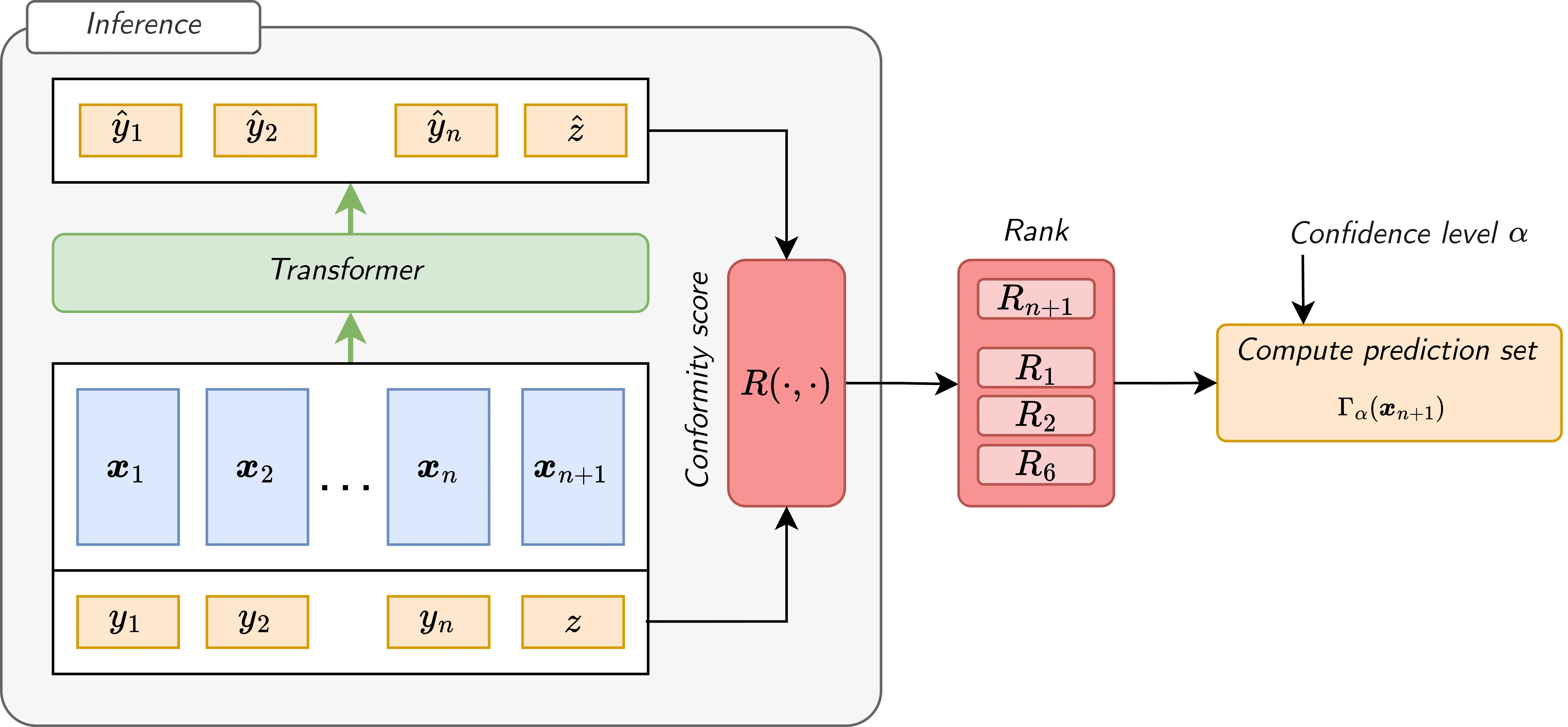
The pretrained parameters remain fixed. We convert these residuals into a typicalness value and retain candidates above the miscoverage threshold :
The prediction region is defined over real-valued responses and targets marginal coverage . Finite-sample validity requires exchangeable context and test data, symmetric score construction, and appropriate treatment of ranks and ties. We use self-attention without a causal mask to preserve the score symmetry. In computation, we evaluate candidates on a finite grid extending 25% of the observed response range beyond each endpoint. The accepted grid values approximate the continuous prediction region; grid resolution and the conversion of accepted values into intervals affect the numerical coverage. Evaluations for different candidates and test inputs are independent and can be batched.
Coverage and computational cost against ridge
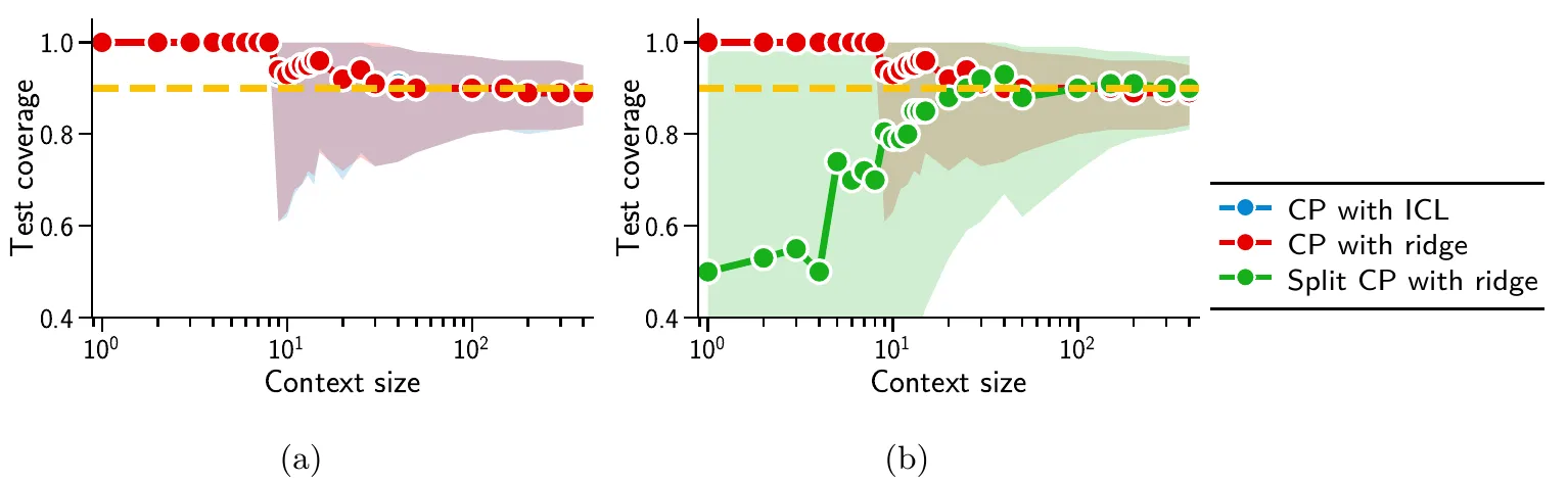
We compare CP with ICL with full CP using ridge and with split CP using ridge. Coverage experiments use 1,000 independent runs, each with context examples and 100 test points; plots report medians and 95% confidence intervals. At , full CP with ICL and ridge approach 90% coverage as context grows. Split CP shows greater variation for small contexts.
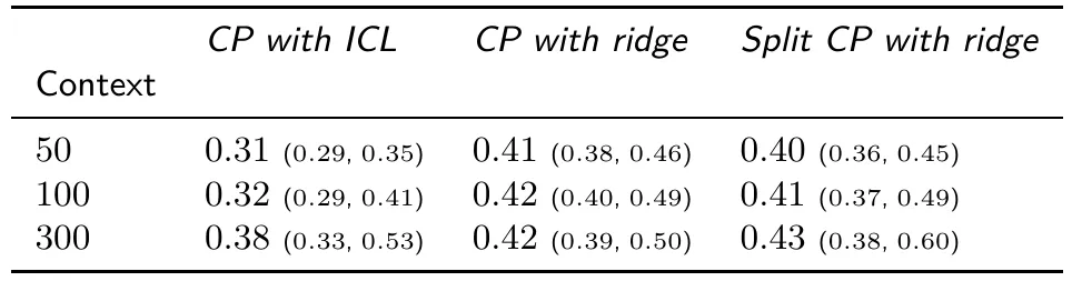
The timing comparison uses the same hardware and optimized, vectorized JAX implementations. At context size 100, median inference times are 0.32 seconds for ICL, 0.42 for full ridge, and 0.41 for split ridge. These measurements cover inference after transformer pretraining.
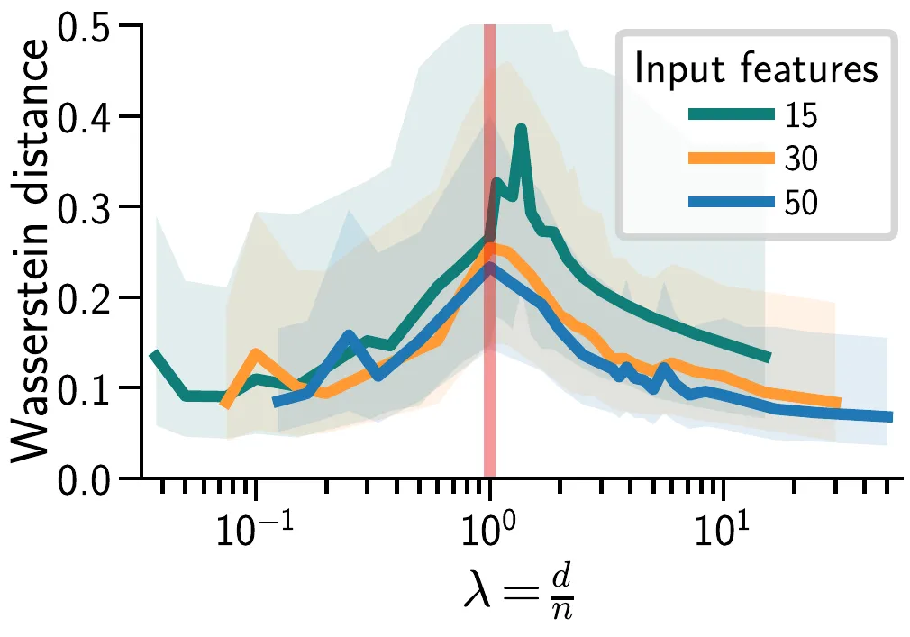
We also compare empirical distributions of typicalness values using Wasserstein-1 distance. This measures agreement between rank-based outputs across candidate evaluations. The discrepancy peaks near , even when coverage remains close to its target.
Shifts from pretraining preserve coverage in the tested tasks
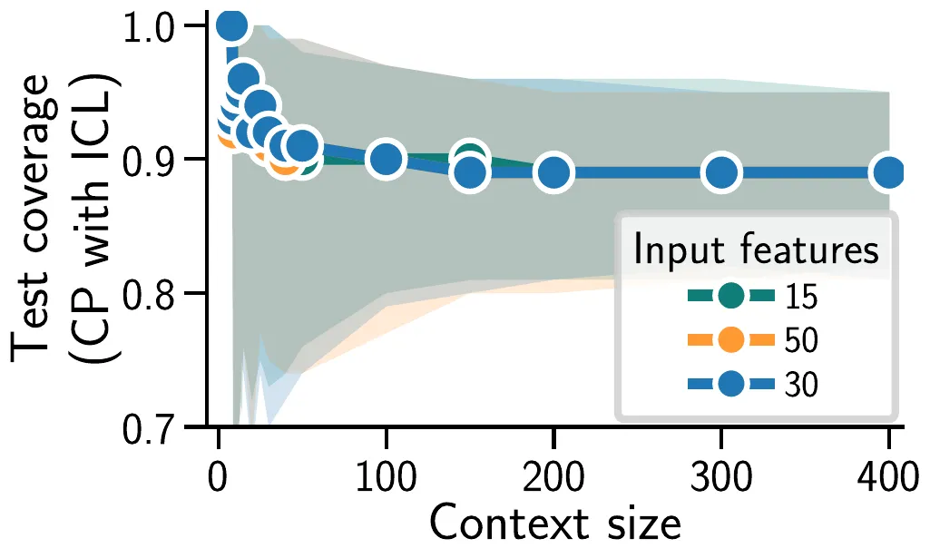
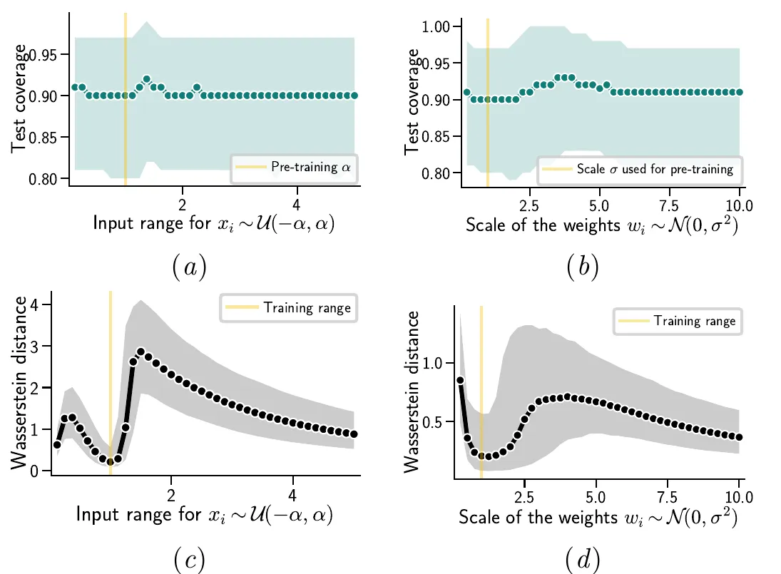
We change the input range or weight scale relative to pretraining, where both equal one. Within each inference task, context and test examples still share a distribution. Coverage remains near 90% across the tested shifts, while typicalness agreement with ridge changes non-monotonically.
Allocating pretraining compute
To study training cost, we fit 40 models at budgets of and FLOPs. We model the Wasserstein discrepancy with
where counts parameters, counts training tokens, and is the fitted asymptotic floor. The coefficients and weight the effects of model size and training data. Here and are scaling exponents, separate from the conformal threshold. The fitted allocation scales as and with compute budget . Two additional models at larger budgets land close to the predicted frontier.
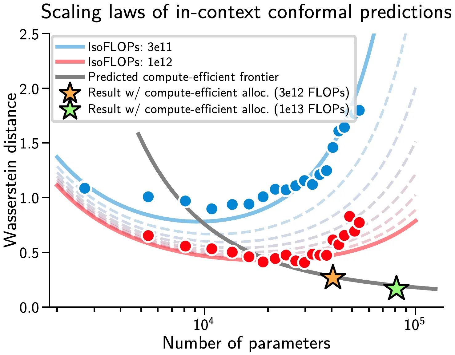
The resulting compute allocation reduces the discrepancy from ridge-based conformal scores within this synthetic regression setting. Prediction-set construction then uses the same frozen non-autoregressive transformer for every candidate response.
Our tumor-segmentation study applies conformal calibration to image regions, separating boundary errors from missed components.